1D Laplace equation - the Euler method

Written on September 7th, 2017 by Slawomir Polanski

The previous post stated on how to solve the heat transfer equation analytically. I could have solved it because the equation form is really simple. For most of the physical problems, it is impossible to find the exact solution of differential equations so scientists have developed numerical methods to get some approximation of what we could obtain analytically. In this blog, I am about to show one of these methods and it is going to be the Euler’s method.

At first, let’s recall the heat transfer problem:

$$\begin{align} \nabla^2 = 0 \Longleftrightarrow \frac{\partial^2 f(x)}{\partial x^2} = 0 \\ x \epsilon [0,1] \quad T(0)=30 \quad T(1)=20 \end{align}$$

The Euler method

Using the definition of function derivative, one can formulate the method as follows:

$$f'(x) = \lim_{h\to0} \frac{f(x+h) - f(x)}{h} \\[1.2em] f'(x) \approx \frac{f(x+h) - f(x)}{h} \Rightarrow f(x+h) = f(x) + hf'(x) \\[1.2em] y_{n+1} = y_n + hf(x_n, y_n)$$

Unfortunately, the specified problem of heat equation is kind of special as it is Double Boundary Value Problem (the two values of temperature are known on the boundaries). To solve it by Euler’s method we need to know a temperature and a derivative of the temperature on one of the boundaries. As I don’t know the derivative, I am going to guess a value and then based on the result check whether it’s correct.

Let’s reformulate the problem to be:

$$\begin{align} \left\{ \begin{array}{l} \frac{dT(x)}{dx} = z\\ \frac{d^{2}T(x)}{dx^{2}} = \frac{dz}{dx} = 0 \end{array} \right. \end{align}$$

In discrete notation it is going to be:

$$\left\{ \begin{array}{l} T_{n+1} = T_n + hz_n\\ z_{n+1} = z_n + hz'_n \end{array} \right.$$

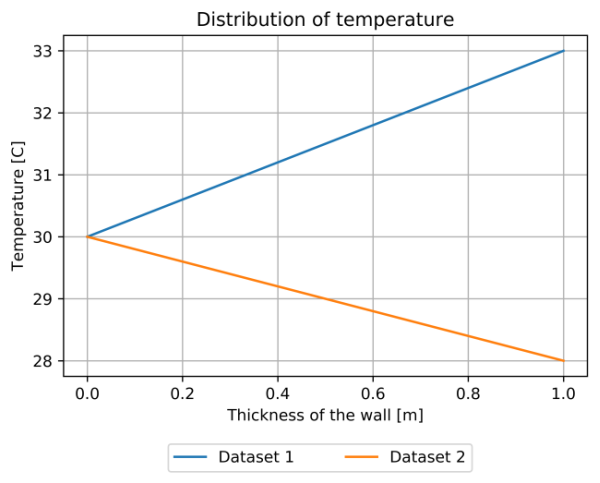
The discrete value of function $T(x)$ is presented below for two datasets:

• Dataset 1: $T(0) = 0$ and $z(0) = 3$
• Dataset 2: $T(0) = 0$ and $z(0) = -2$

One can see that the values for the second dataset are getting lower through the wall thickness and it is more suitable for our example. Now, we can take another shoot and try to hit $T(1)=15$, but it is better to take advantage of following formula:

$$\begin{align} z_{exact} = z_{1} + \dfrac{z_{2} - z_{1}}{(T_{2}(1) - T_{1}(1))(T(1) - T_{1}(1)} \\ = 3 + \dfrac{-2 + 3}{(-2 - 3)(15 - 3)} = -15 \end{align}$$

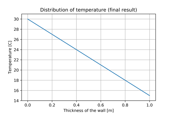
Knowing that $T(0) = 0$ and $\frac{dT(x)}{dx} = -15$ we can obtain the final solution.

Summary

This time, the method used for obtaining a solution seems to take more time than analytical way. In the next post I will present how to solve 1D Poisson’s equation and this will prove how handy the numerical methods are. For those who might be interested, I am attaching also the Python code which I used to get results.

SP