1D Laplace equation - Analytical solution

Written on August 30th, 2017 by Slawomir Polanski

The Laplace equation is one of the simplest partial differential equations and I believe it will be reasonable choice when trying to explain what is happening behind the simulation’s scene. Despite it’s simplicity, the equation can be used to understand various engineering and scientific problems, for instance:

• steady-state temperature distribution (heat conduction analysis)
• steady-state stress distribution (rod under torsion load)
• potential flow
• electrostatics and electromagnetism

In this article, I will solve one-dimensional steady-state heat conduction problem analytically. The equation will take form of Ordinary Differential Equation, but it is good introduction before moving on to bigger things. In the next post I am will try to present how to obtain the same results numerically.

Analytical solution

In one dimensional space, the equation can be written as:

$$\nabla^2 = 0 \Longleftrightarrow \frac{\partial^2 f(x)}{\partial x^2} = 0$$

In order to solve it, both left and right side has to be integrated.

$$\begin{align} \int \frac{\partial^2 f(x)}{\partial x^2} dx &= \int 0\, dx \\[0.5em] \int \frac{\partial f(x)}{\partial x} dx &= \int C_1\, dx \\[0.5em] f(x) &= C_1 x + C_2 \end{align}$$

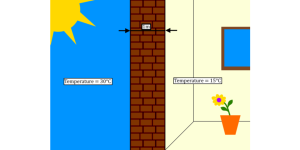
In case of heat equation, it is better to write the function $f(x)$ as $T(x)$ as it logically corresponds to the temperature distribution. Also, to understand the heat conduction better, let’s refer to this super-scientific sketch below. Our aim is to find out how the temperature is going to change in the wall.

Assuming that $x=0$ for the outside surface of the wall and $x=1$ for inner side:

$$\begin{align} x \epsilon [0,1] \quad T(0)=30 \quad T(1)=15 \end{align}$$ $$\left\{ \begin{array}{l} 30 = C_1 \cdot 0 + C_2 \Rightarrow C_2 = 30\\ 15 = C_1 \cdot 1 + C_2 \Rightarrow C_1 = -15 \end{array} \right. \\[1.2em] T(x) = -15x + 30$$

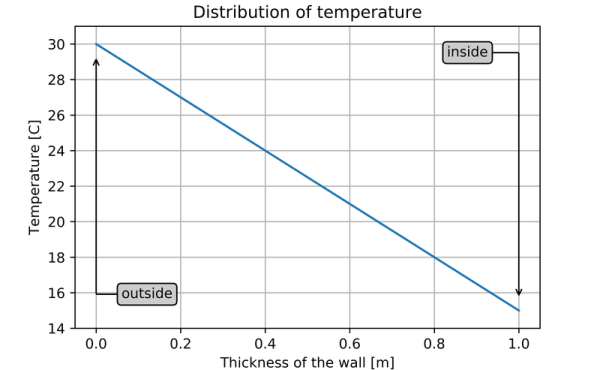
Using the obtained function $T(x)$, we can plot following graph.

Summary

OK, I admit…The solution isn’t spectacular and it was easy to guess the temperature distribution without solving all these integrals and differential equations… Still, I believe it is a good point to start learning the background of numerical simulations. I will post soon how to solve the equation using Euler method.

SP